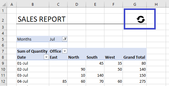
Refresh All Button
It’s easy to forget to refresh your Pivot Tables when you add new source data. Here’s an effective solution to that problem: Add a Refresh button in your Excel report!

This is very easy, and only takes a minute:
There are 3 steps:
Step 1:
Go to the Insert menu, choose Icons and type “Refresh” in the search field. Choose the icon you want, and click on Insert. Resize and place the icon where you want to have it.

Step 2:
Open the VBA editor (Alt + F11). Go to the Insert menu and choose Module. Type this code:
Sub RefreshAll()
ActiveWorkbook.RefreshAll
End Sub
Step 3:
Go back to Excel, right-click on the Refresh Icon and choose “Assign Macro”. Choose the “RefreshAll” macro and click OK.
The next time you add data to your Pivot Table, or you want to get the most recent data from your Datawarehouse, simply click on your new Refresh button!
Important: When you save the workbook, you need to save it as either Excel Macro-Enabled Workbook or Excel Binary Workbook!
BONUS TRICK:
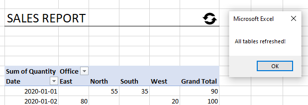
Add one more line to the code and get a popup message when the refresh is done:
Sub RefreshAll()
ActiveWorkbook.RefreshAll
MsgBox “All tables refreshed!”
End Sub
Of course, you can write any text you want between the double quotes.

Recommended Articles
This has been a guide to Basic Formulas in Excel. Here we discuss the list of top 10 Basic Formulas & Functions in Excel, including SUM, COUNT, COUNTA, COUNTBLANK, MAX, MIN, etc. with a downloadable excel template. You may learn more about excel from the following articles –
- Excel IF Formula
- Average Formula
- How to use Mode Function in Excel?
- VBA TRIM Examples
Further reading:
Basic concepts
Getting started with Excel
Cell References


