Home Excel Tips and Tricks Conditional Formatting for a row

Conditional Formatting for a row

Conditional Formatting For A Row

You are going to learn, how to format whole row not only one cell. It can be useful for some reports or presentations.

Format row formatted

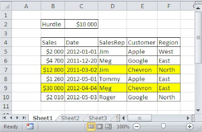
You have some sales report.

Format row sales report

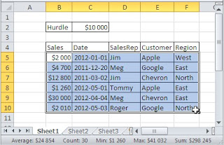
You can format rows, which sales is more then 10 000$. First select your data without headings.

Format row select data

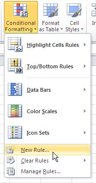
Next go to the ribbon and click Conditional Formatting and New Rule.

Format row new rule ribbon

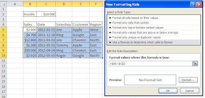
On the dialog box choose Use a formula to determine which cells to format option.

Format row new rule

Write down =$B5>$C$2 formula.

Format row formula

Next click Format and choose how your rows will be formatted. I clicked Fill and chose yellow background.

Format row fill

Click OK and see you data formatted? Conditional Format row

This is how Conditional Formatting for a row is working. Isn’t it easy?

You can download the Template here – Download

Further reading: 
Basic concepts 
Getting started with Excel
Cell References