Conditional formatting in Excel
Basic formatting
I prepared a table with the results of the exam.
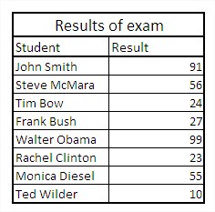
You want to highlight the extreme results. The best results are above 90% mark in green, and below 30% in red. How to do it?
Conditional formatting button is at the center of the Excel ribbon.
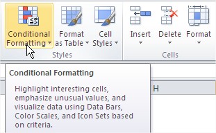
Start with the best students. All results above 90% want to paint the green. Click on the button Conditional Formatting on the ribbon and select Greater Than….

A dialog box appears. The entry requirement of 90% and selecting the format of a custom list to determine the green fill.
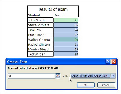
Similarly do with next conditions. For results less than 30% choose to fill the red. The results look as follows:

Excel automatically formats all cells according to the given condition.
Advanced formatting
Other (example) formatting options presented in the following figure.
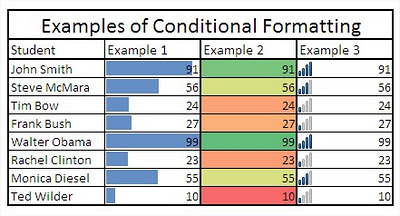
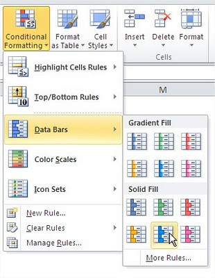
I marked the first column with blue stripes. The higher the number in the cell, the longer the formatting toolbar. This option can be turned on in a way that I showed in the picture.
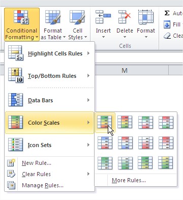
The second column formatting benefited from the color scale. Only the first scale – the highest values are green and red the lowest.
Results in the third column formatted sets of icons. I think this is a good way to spice up the sheet, but for use at work is not the best idea.
![]()
There are many more possibilities. Try them all at home.
Template
Further reading:
Sorting
Conditional Formatting for a row
How to Format Date and Time?


