How To Change The Color Of Markers On A Chart in Excel
 2. Select the marker upon right click a dropdown appear. Then select the Format Data Series option.

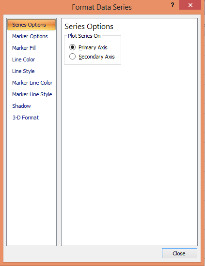
3. A window will appear like this below.

4. Select the Marker Fill option from left side and choose Solid Fill and from the colors. Select the new color of the marker.

5. Now here you go with changed color of your marker.

Remember that the chart should be first of all easy to read for people who will use it. Color of marker should be distinct from the color of the line. Excel offers you whole range of colors to set. You can choose whatever colors you want.
Template
You can download the Template here – Download


