Case Sensitive VLOOKUP

Case-sensitive vlookup

Vlookup function doesn’t care about case-sensitivity. So what to do when you do?

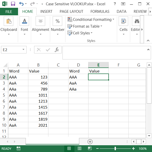
This is an example:

The task is to vloookup the value to the word. Formula should care about case-sensitivity.

The solution is this array formula:

=VLOOKUP(value,IF(EXACT(value,column),table),column_number,0)

0 here means the exact match for the vlookup function.

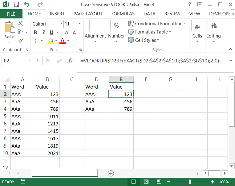
Formula in the example is:

{=VLOOKUP($D2,IF(EXACT($D2,$A$2:$A$10),$A$2:$B$10),2;0)}

Please be aware that it is an array formula so you need to use CTRL + SHIFT + ENTER keyboard shortcut. That’s why there are braces around the formula. They appears after you typed CTRL + SHIFT + ENTER.

Case-sensitive lookup

The problem is that your data differ only by case so capitalization is important for you. That’s why you need case sensitive lookup. Let’s construct a formula which will solve your problem. INDEX formula suits the best. Syntax here will be:

=INDEX(value_you_need, row_number, column_number)

• value_you_need is a data range from your data table
• row_number – this is hard to get. You have to use EXACT function for case sensitive function
• column_number is always 1

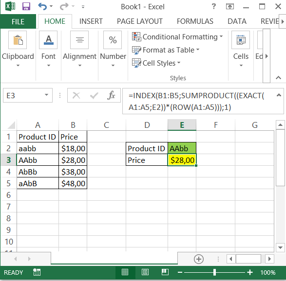
In this example you need the Price and you have Product IDs. The formula you need is:

=INDEX(B1:B5;SUMPRODUCT((EXACT(A1:A5;E2))*(ROW(A1:A5)));1)